- Original article
- Open access
- Published:
The Balassa-Samuelson effect reversed: new evidence from OECD countries
Swiss Journal of Economics and Statistics volume 155, Article number: 3 (2019)
Abstract
This paper reconsiders the Balassa-Samuelson (BS) hypothesis. We analyze an OECD country panel from 1970 to 2008 and compare three data sets on sectoral productivity, including newly constructed data on total factor productivity. Overall, our within- and between-dimension estimation results do not support the BS hypothesis. For the time since the mid-1980s, we find a robust negative relationship between productivity in the tradable sector and the real exchange rate, even after including the terms of trade to control for the effects of the home bias. Earlier, supportive findings may depend on the choice of the data set and the model specification.
1 Introduction
The Balassa-Samuelson (BS) hypothesis—stated by both Balassa (1964) and Samuelson (1964), with a research precedent in the work of Harrod (1933)—is one of the most widespread explanations for structural deviations from purchasing power parity (PPP)Footnote 1.
According to the BS hypothesis, differences in the productivity differential between the non-tradable and the tradable sector lead to differences in price levels between countries when converted to the same currency. The hypothesis assumes that the law of one price for tradable goods holds. Ceteris paribus, a productivity increase in tradables raises factor prices, i.e., wages, which in turn leads to higher prices of non-tradables and thus to an appreciation of the real exchange rate. In contrast, when the relative productivity of non-tradables increases, marginal cost cuts result in a lower price level.
The empirical evaluation of the BS hypothesis has gained a great deal of attention. As argued in a survey by Tica and Družić (2006), the major share of the evidence supports the BS model, but the strength of the results depends on the nature of the tests and set of countries analyzedFootnote 2. In particular, cross-sectional studies have been more successful in finding support for the BS hypothesis than panel data studies.
There are, however, several studies based on a disaggregation of the tradable and non-tradable sector that find empirical support for the BS hypothesis (see, e.g., Calderón (2004); Choudhri and Khan (2005); Ricci et al. (2013) or Berka et al. (2018)). In particular, since sector-specific data for OECD countries on total factor productivity (TFP) have become available, various studies have tested and confirmed the BS hypothesis using panel data (De Gregorio et al. 1994; De Gregorio and Wolf 1994; Chinn and Johnston 1996; MacDonald and Ricci 2007). All these studies are based on the discontinued International Sectoral Database (ISDB) provided by the OECD.
This paper applies two panel cointegration models to estimate the long-run relationship between the real exchange rate and key explanatory variables, focusing on the effect of the TFP differential between tradables and non-tradables. Panel cointegration methods have become increasingly important in testing the BS hypothesis (Tica and Družić 2006). We use a novel OECD data set (PDBi) with annual sector-specific TFP data from 1984 to 2008 to eliminate some of the shortcomings of the ISDB.
With this new data set, our estimations cannot confirm the broad-based findings of previous research based on the ISDBFootnote 3. In fact, the results point to a negative relationship between tradable productivity and the real exchange rate for OECD countries. In other words, for the time since the mid-1980s, an increase in the productivity of tradables has given rise to a depreciation of the real exchange rate. This finding is the opposite of what is claimed by the BS hypothesis, but it is in line with the empirical evidence for OECD countries documented by Égert et al. (2006) and Fazio et al. (2007). Our analysis, however, differs from these studies in a number of dimensions, including the estimation methodsFootnote 4, the data set, the sample period, and the set of OECD countries analyzed. Importantly, while these authors find a statistically significant negative relationship between the labor productivity of tradables and the real exchange rate, our analysis also relies on sector-specific TFP, which is the preferred measure for productivity as noted by De Gregorio and Wolf (1994)Footnote 5. However, we can confirm this result when TFP is replaced by labor productivity (LP) using the OECD Structural Analysis (STAN) data set, which covers more countries and a longer time period, from 1970 to 2008. A rigorous analysis reveals that the finding of a negative coefficient on the productivity in the tradable sector for the time since 1984 is robust against the choice of the productivity measure (TFP or LP), the choice of the country sample, the precise start of the sample period, the exact model specification, and the inclusion of additional explanatory variables. Moreover, it seems that the negative effect of tradable productivity on the real exchange rate has strengthened over time. Our analysis further indicates that the choice of the model specifications matters for the finding as to whether the empirical relationship between the productivity of tradables and the real exchange rate is negative or positive for the time period from 1970 to 1992, using the ISDB.
So far, the literature has primarily proposed deviations from the law of one price, such as a home bias in consumption preferences, as a possible mechanism for this reversed BS effectFootnote 6. Benigno and Thoenissen (2003) develop a new open economy model in which a TFP shock in the tradable sector weakens the real exchange rate because the effect of the decrease of the price of its traded goods relative to that abroad dominates the effect of the increase of the relative price of non-traded goodsFootnote 7. More recently, Berka et al. (2018) provide a detailed breakdown of the real exchange rate based on a New Keynesian model. In particular, they show that the traded goods real exchange rate depends on three factors: (1) differences in relative non-traded goods prices across countries capturing distribution costs, (2) terms of trade (ToT) capturing home bias in preferences, and (3) deviations from the law of one price as deviations between the foreign price of identical goods relative to the home price. Thus, the authors distinguish between the effects of ToT and the explicit law of one price and assume that the latter holdsFootnote 8. We adopt this assumption because the aggregation level of our data set does not allow us to consider this third factor in the estimations. Berka et al. (2018) then show that relative non-tradable productivity, relative tradable productivity, and ToT drive the overall real exchange rate. Therefore, we use ToT to control for the impact of movements in relative export to import prices on the real exchange rate. However, the inclusion of ToT does not change the significant negative relationship between the productivity of tradables and the real exchange rate. This result suggests that a productivity increase in the tradable sector can lead to a decrease in the relative price of non-traded goodsFootnote 9. Gubler and Sax (2014) provide a static general-equilibrium framework with skill-based technological change (SBTC), in which higher productivity in the tradable sector can lower wages, which in turn leads to lower prices of non-tradables and thus to a depreciation of the real exchange rate. Berka et al. (2018) show that ToT are closely related to the relative unit labor costs (ULC) and propose to replace ToT with unit labor costs because the use of the ToT raises conceptual and empirical difficulties. Therefore, we replace ToT with ULC in a robustness check. The negative relationship between tradable productivity and the real exchange rate remains in force.
On the other hand, the connection between non-tradable productivity and the real exchange rate is not robust. Our robustness tests reveal that severe outlier dependency exists for the traditional Balassa-Samuelson finding regarding non-tradables. In particular, Japanese labor productivity in the non-tradable sector strongly weakens the estimated BS effect. For the time period from 1970 to 1992, the coefficient even significantly changes its sign once Japan is included.
Finally, with the exception of the terms of trade, our estimation results indicate that the explanatory power of further control variables discussed in the literature is weak or not robust.
The remainder of this paper is organized as follows. Section 2 presents the data. We outline the methodology in Section 3 and show the results in Section 4. Section 5 concludes.
2 Data
The data for the 18 major OECD countries included in our data set stem from different data sets of the IMF, OECD, World Bank, and the Penn World Tables. Depending on the estimation, the country sample has to be reduced mainly because not all data are availableFootnote 10. A detailed description of all variables is given in Table 1 and in Appendix 1.2.
To test the BS hypothesis, we condition the real exchange rate on productivity measures for both the tradable and the non-tradable sector as well as on control variables. The choice of the dependent variable is discussed in Section 2.1. Due to its importance and complexity, the productivity data are separately examined in Section 2.2. All other exogenous variables are discussed in Section 2.3. The time series properties of the variables are assessed in Section 2.4.
2.1 Dependent variable: real exchange rate
We use the logarithm of the unweighted real exchange rate (RER) as the dependent variable in our estimation equations and define it such that an increase represents an appreciation. In principle, the real exchange rate can only be computed towards a reference currency. However, since we use time fixed effects throughout our analysis, the choice of the reference currency does not impact the resultsFootnote 11. Like for all variables in our analysis, the inclusion of time fixed effects is equivalent to subtracting the annual sample mean. This is also true in the presence of DOLS estimators, when differences of variables are used in the regression. In this case, the inclusion of time fixed effects is equivalent to subtracting the annual sample mean of the difference. The advantage of not using a reference country is that it allows us to keep all available countries in the sample.
An extensive body of the empirical literature uses effective real exchange rates (see, e.g., De Gregorio and Wolf (1994); Calderón (2004) or Ricci et al. (2013)) that are weighted by the share of exports. Effective real exchange rates have the advantage that there is no need to specify a reference country. While effective real exchange rates are a useful measure for competitiveness, the share of exports seems not only irrelevant in our context but also misleading. If, for example, a country changes its export destinations to countries with a weaker real exchange rate, effective real exchange rates would indicate a real appreciation, while, in fact, the country still has the same relative price level towards all countriesFootnote 12.
2.2 Productivity data
We use data on sectoral productivity from three data sets provided by the OECD. The first is a new data set on sectoral total factor productivity (TFP) computed by the OECD, called PDBi. PDBi extends the older PDB by providing annual sector-specific TFP numbers for the time period from 1984 to 2008. Sectoral TFP is calculated as Solow residuals with the same method for all countries, using sectoral data on production, employment, capital stock, and the labor share of income. Capital stocks are estimated by applying the permanent inventory method, where streams of investments are added, and a certain fraction of depreciation is subtracted each year (for more details, see Arnaud et al. (2011)).
A second data set, STAN, includes yearly data on sectoral production and employment—and thus on labor productivity—but not on TFP. As the only data set, STAN covers a long time range, from 1970 to 2008, for many OECD countries.
To compare our findings with the existing studies (De Gregorio et al. 1994; De Gregorio and Wolf 1994; Chinn and Johnston 1996; MacDonald and Ricci 2007), sectoral productivity data from the discontinued ISDB have been used as well. This old data set contains annual values on labor and total factor productivity—in principle from 1970 to 1997—but was discontinued before 1997 for most countries.
STAN and PDBi data are improvements to the ISDB. In the old data set, output, employment, and capital stocks were based on data from an old system of national accounts, SNA68. For social services, these changes in the measurement of output may have been especially important because the estimates of the real value added growth for the public sector in the ISDB have simply been based on labor inputs such that the estimates of productivity had very limited meaning. Moreover, in the ISDB, volumes were calculated using constant prices instead of chain-linking. Finally, capital stock estimates may have been calculated differently and in a non-standardized way in the ISDBFootnote 13.
We use these three OECD data sets for the following reasons: first, sectoral productivity data from PDBi has, to our best knowledge, not yet been used in testing structural deviations from purchasing power parity (PPP). Second, it allows us to compare our results, which are based on STAN and ISDB, with several important contributions to the literature on the BS hypothesis. Third, our approach also allows us to shed some light on whether differences in the results stem from the choice of the productivity measure (TFP or LP), the estimation period or the choice of the data set. In addition, important control variables such as the terms of trade or unit labor costs also stem from OECD databases.
The classification of the subsectors into tradable and non-tradable is done according to the following scheme: agricultureFootnote 14, manufacturing, and transport, storage, and communications are classified as tradables; utilities (energy, gas, and water), construction, and social services (community, social, personal services) are non-tradables. Our division of the subsectors into tradable or non-tradable sectors follows De Gregorio and Wolf (1994), who defined a subsector as tradable if its share of exports in the total production exceeds 10% and as non-tradable otherwiseFootnote 15. While no division has become standard in the field (Tica and Družić 2006), studies based on data from OECD countries usually refer to the division proposed by De Gregorio and Wolf (1994) (see, e.g., Chinn and Johnston (1996); MacDonald and Ricci (2007)). Like MacDonald and Ricci (2007), we exclude mining and business servicesFootnote 16 due to data availability and the distribution subsector (wholesale and retail trade) due to classification difficulties. Based on a simple theoretical model, MacDonald and Ricci (2005) show that an increase in the productivity of the distribution subsector can have an ambiguous effect on the real exchange rate because of its role in delivering intermediate inputs to firms and final goods to consumersFootnote 17.
The tradable and non-tradable sectors, when classified this way, are roughly equal in terms of the value added. Within the tradable sector, manufacturing is by far the largest subsector, representing 64% of the value added, whereas agriculture and transport as well as storage and communications amount to 11% and 24%, respectively. Among the non-tradables, social services (70%) outweigh construction (20%) and utilities (9%). Figure 2 in Appendix 1 displays the data availability in each of the three data sets.
Table 2 shows the correlations between the three data sets. The LP and TFP values from the ISDB are similar to the two newer data sets only in the tradable subsectors. In the non-tradable sectors, the correlations are lower (construction and utilities) or virtually non-existent (social services). To a lesser extent, this is also true for employment and value added. Possible reasons for these divergences have been discussed earlier in this section. On the other hand, the data from the PDBi on TFP are highly correlated with labor productivity from the STAN data set. These correlations are present in all subsectors, although the values are somewhat lower in the non-tradable subsectors. TFP data from ISDB and PDBi shows the lowest correlations. But again, the correlations are relatively high for agriculture and manufacturing, the main tradable sector. Unfortunately, there is only a low number of time-overlapping observations on TFP from the PDBi and ISDB (see Figure 2 in Appendix 1), which may explain this result to a relevant extent.
We consider TFP to be the preferred measure for productivity. As noted by De Gregorio and Wolf (1994), the average labor productivity increases much more quickly during economic downturns; hence, it is not a reliable indicator of sustainable productivity growth, which can affect the economy in the medium or long term. Nevertheless, there are some advantages of LP, and we will use the measure to check the robustness of our TFP resultsFootnote 18.
2.3 Control variables
Along with the data on sectoral productivity, we take into account further potential determinants of the long-run real exchange rate, which have been proposed in the literature. As described by De Gregorio and Wolf (1994) or Sax and Weder (2009), among others, an improvement in the terms of trade (TOT) allows a country to raise its imports for a given number of factor inputs in the export sector. For example, a change in consumer preferences may shift global demand towards a specific country’s export goods. As a result, the good’s global price increases and, hence, the country’s real exchange rate appreciates. Moreover, supply side changes may also affect the real exchange rate through movements in the terms of trade, for example, due to the home bias in consumption preferences (see, e.g., Benigno and Thoenissen (2003); MacDonald and Ricci (2007), Choudhri and Schembri (2010) or Berka et al. (2018)). Berka et al. (2018) show in a New Keynesian model that the terms of trade are closely related to the relative unit labor costs (ULC). They propose to replace the terms of trade with unit labor costs because the use of the former raises conceptual and empirical difficulties. Unit labor costs are given as the ratio of total labor compensation per hour worked to output per hour worked, and are thus directly comparable between countries. Most importantly, the terms of trade and the real exchange rate are endogenous relative prices and so they are simultaneously determined. Therefore, we use ULC to replace TOT in a robustness analysis.
Several authors note the importance of further demand-side factors for the determination of the long-run real exchange rate. Therefore, we consider the government spending share (GOV), net foreign assets (NFA) relative to GDP, the current account relative (CA) to GDP and real GDP per capita (GDP) as control variables.
De Gregorio and Wolf (1994) show theoretically that an increase in government spending causes the equilibrium real exchange rate to appreciate if capital mobility across countries is restricted. This increase affects the relative price of tradable and non-tradable goods negatively because government spending tends to fall more heavily on non-tradables. Hence, government spending is widely used as an additional explanatory variable (see, e.g., Chinn and Johnston (1996); Sax and Weder (2009) or Ricci et al. (2013)).
Private demand may affect the real exchange rate as well. It is likely that a higher income is associated with a higher demand for non-tradables. The associated rise in the relative price of non-tradables gives rise to a higher overall price level (De Gregorio and Wolf 1994). Furthermore, trade deficits or surpluses could affect the demand for non-tradables by increasing or decreasing the amount of tradables that are available for consumption. As a permanent trade deficit can only be sustained in the presence of net foreign assets, several authors have emphasized the importance either of the net foreign assets or the current account deficit for the determination of the real exchange rate (Krugman 1990; Lane and Milesi-Ferretti 2004; Ricci et al. 2013).
Finally, two other macroeconomic variables, the real interest rate (RI) and the population growth rate (DPOP), are taken into account. Their importance for the determination of RER has been discussed in theoretical and empirical contributions to the literature. According to the theoretical model provided by Stein and Allen (1997), a higher real interest rate is associated with an appreciated long-run real exchange rate because of portfolio adjustments and capital inflows. Rose et al. 2009 show in an overlapping generation model that a country experiencing a decline in its fertility rate will also experience a real exchange rate depreciation. We use population growth as a proxy for fertility rates.
2.4 Assessing the time series properties of the variables
The panel unit root tests proposed by Levin et al. (2002) (LLC) and Im et al. (2003) (IPS) have been conducted for all variables (Table 3). To obtain reliable results, the test statistics are based on all available information for both time and cross-sectional dimensions. The real exchange rate is calculated for every year towards the annual average of the sample (denoted RER.AVG)Footnote 19.
Overall, we find strong evidence for non-stationary behavior for all variables, with the exception of the population growth rate, DPOP. Because DPOP is the first difference of the logarithm of the population, this result is not surprising. Unit labor costs show ambiguous results. The same holds for the total factor productivity in the tradable sector from the PDBi data set (TFP.TPDBi) and labor productivity in the tradable sector from the STAN data set (LP.TSTAN). However, the non-stationarity of these variables is confirmed by the Fisher-type augmented Dickey-Fuller (ADF) panel unit root test proposed by Maddala and Wu (1999) and Choi (2001) (results not shown)Footnote 20. Moreover, Harris et al. (2005) and Pesaran (2007) also provide evidence for the failure of purchasing power parity when allowing for cross-section dependence between the real exchange rates in a panel of OECD countries. All results are also in line with the results found in similar empirical studies (see, e.g., Calderón (2004); MacDonald and Ricci (2007) or Ricci et al. (2013)).
3 Methodology: cointegration tests and panel DOLS
The number of observations for each country is limited given the length of the sample (23 years in our benchmark model) and the annual data frequency. Therefore, we pool the data and apply a panel estimation technique to improve the power of our results. We are primarily interested in the long-run relationship between the real exchange rate and its determinants, which are described in Section 2 and summarized in Table 1. To estimate this relationship, we employ a panel cointegration model that treats the non-stationarity of the variables correctly.
Our results are based on the within-dimension dynamic ordinary least squares (DOLS) estimator. Several methods to estimate a panel cointegration model are discussed in the literature. However, Kao and Chiang (2001) show that the DOLS approach developed by Stock and Watson (1993) outperforms the panel OLS or the fully modified OLS (FMOLS) procedures in the sense that the DOLS estimator is less biased in finite samples. In addition, the choice of this method facilitates a comparison with the results from similar studies, e.g., Ricci et al. (2013), MacDonald and Ricci (2007) and Fazio et al. (2007). Our estimation equation has the following form:
where RERit denotes the real exchange rate at time t of country i, αi is a country fixed effect, δt is a time fixed effect, Xit is a vector containing the explanatory variables, β is the cointegration vector, k and p are the maximum and minimum lag lengths, respectively, γj are the k+p+1 vectors containing the coefficients of the leads and lags of changes in the explanatory variables, and εit represents the error term. The inclusion of the leads and lags solves the potential endogeneity problem by orthogonalizing the error termFootnote 21.
Time and country fixed effects are included to reduce the omitted variable bias and to solve the problem that some variables are indices; hence, their levels are not comparable across countries. Furthermore, as described in Section 2.1, time fixed effects allow us to abstain from the use of a reference country when computing real exchange rates.
We report standard errors developed by Driscoll and Kraay (1998) that are robust to very general forms of spatial and temporal dependence. For the computation, we follow Cribari-Neto (2004), who proposed an estimator (called HC4) that is reliable when the data contain influential observationsFootnote 22.
To ensure that what we find is indeed a long-run relationship between the real exchange rate and the set of explanatory variables, we test for cointegration using two methods. First, we follow MacDonald and Ricci (2007), who apply the standard unit root test of Levin et al. (2002) to the estimated residualsFootnote 23. Second, we employ the Kao (1999) panel cointegration test. Since this test requires a balanced panel, some observations have to be dropped; therefore, the test is mainly applied to check the robustness of the first test results.
Moreover, to allow for more flexibility in the presence of the heterogeneity of the cointegrating vectors, we employ the between-dimension group-mean panel FMOLS estimator from Pedroni (2001)Footnote 24. This method has the additional advantage that the point estimates can be interpreted as the mean value for the cointegrating vectors and that the estimator exhibits smaller size distortions in small samples.
4 Empirical results
To explore the validity of the Balassa-Samuelson (BS) hypothesis, we estimate various within-dimension DOLS model specifications and employ the between-dimension group-mean panel FMOLS estimator from Pedroni (2001).
This section presents the results for the long-run relationship between the real exchange rate and relative productivity as well as the control variablesFootnote 25. Therefore, we provide an extensive robustness analysis of our main findings. In addition, the results of the cointegration tests described in Section 3 are reported.
4.1 The Balassa-Samuelson effect from the 1970s to the 1990s
Since sector-specific data for OECD countries on total factor productivity (TFP) have become available through the release of the discontinued International Sectoral Database (ISDB) by the OECD, various studies have tested the BS hypothesis in panel data for the years after Bretton Woods. Among others, MacDonald and Ricci (2007) find a statistically significant BS effect on the real exchange rate of OECD countries in panel estimations.
As a first step, we examine the robustness of the BS effect with respect to the use of the productivity measure (labor productivity (LP) or TFP), the choice of the data set, and the model specification. For this purpose, we conduct a similar exercise as, e.g., MacDonald and Ricci (2007). Therefore, the real exchange rate (RER) is first conditioned on total factor productivity of tradables (TFP.T) and non-tradables (TFP.NT), net foreign assets (NFA) relative to GDP, and the long-term real interest rate (RI) for the period from 1970 to 1992. The countries considered are listed in sample (i) in Appendix 1.1.
Column (1) of Table 4 reports the results with TFP data from the ISDB and, in line with MacDonald and Ricci (2007), adding three leads and lags of the first-differenced explanatory variables to the estimation equation. Except for RI, the results are qualitatively equal to the findings of MacDonald and Ricci (2007). In particular, the signs of the coefficients related to both TFP variables are consistent with the BS hypothesis. Quantitatively, though, the effects of TFP.TISDB and TFP.NTISDB on the real exchange rate are somewhat stronger. Overall, we also find the results in favor of the BS theory with data from the ISDB.
However, the successful confirmation of the BS hypothesis may depend on the use of the productivity measure. As described in more detail in Section 2.2, there are some advantages of LP, and we will use this measure to check the robustness of our results with TFP. Column (2) shows that, all else being equal, the use of LP instead of TFP from the ISDB has only a minor impact on the effect of productivity in the tradable sector on RER, while the effect of productivity in the non-tradable sector on RER vanishes.
As a second robustness check, we also estimate the model with labor productivity from a different data set, STANFootnote 26. In contrast to the discontinued ISDB, STAN allows us to extend the sample period to 2008 and thus link the findings of this section with those in Section 4.2. As displayed in column (3), for the period 1970 to 1992, the coefficient on LP.TSTAN is positive and statistically significant, confirming the previous results. However, the use of STAN lowers the magnitude of the effect by half. The coefficient on LP.NTSTAN becomes positive and is highly statistically significant, contradicting previous results and the BS hypothesis. This result mainly reflects differences in the computation of labor productivity of social services (community, social, personal services) across the two data sets (see Table 2 in Section 2.2). Group-mean panel FMOLS estimates show that Japan seems to be an outlier that critically affects the estimation of the coefficient for productivity in the non-tradable sector. While an increase in labor productivity in the non-tradable sector gives rise to a significant real exchange rate appreciation, the contrary is true if Japan is omitted (results not shown).
As a third robustness check, we test the impact of the choice of the number of leads and lags on the estimation results. The use of three leads and lags considerably reduces the number of de facto observations. This may be a caveat, particularly in samples with a relatively small numbers of years. Therefore, column (4) shows the estimation results with TFP data from the ISDB and applying one lead and lag. In this case, the effect of productivity in the tradable sector on RER becomes much smaller and statistically insignificant. The coefficient on TFP.NTISDB slightly decreases but remains statistically significant.
Finally, we employ a group-mean panel FMOLS estimator (Pedroni 2001) to the same data set. Abandoning the assumption of a common value under the alternative hypothesis has a major effect on the coefficient TFP.TISDB (column (5)). Productivity in the tradable sector affects the real exchange rate significantly negatively. Only for Norway do we find a statistically significant positive effect, supporting the BS hypothesis. The estimated effect of productivity in the non-tradable sector on RER is much smaller than in the within-dimension DOLS model estimation (column (1)) but remains in line with the BS hypothesis. For six countries, TFP.NTISDB is significantly negative, while TFP.NTISDB is significantly positive for only two countries.
Overall, the results suggest that there is only weak evidence for the BS hypothesis. The results are not robust to several modifications along the various dimensions. In particular, the positive relationship between tradable productivity from ISDB and the real exchange rate may depend on the choice of the model specification. In contrast, the negative relationship between non-tradable productivity and the real exchange rate seems to be more sensitive to the choice of the data set and, to a lesser extent, to the definition of productivity. This is not surprising given the difficulty of computing productivity values for the subsectors defined as non-tradables (see Section 2.2), since (real) output and prices are often not directly observable.
In line with MacDonald and Ricci (2007), the control variables NFA and RI mostly have the theoretically correct sign, but the economic effect is rather small and rarely statistically significant. The coefficient NFA is considerably smaller compared to the results of Lane and Milesi-Ferretti (2004). Similarly, Ricci et al. (2013) also find an economically small and insignificant effect of net foreign assets (relative to trade) on the real exchange rate of advanced countries.
4.2 The Balassa-Samuelson effect in recent times
The OECD provides a novel data set (PDBi) with sector-specific TFP data, which eliminates some of the shortcomings of the ISDB data set. Moreover, the new data set covers more recent times.
While examining the validity and robustness of the BS hypothesis using data from PDBi, we choose the number of leads and lags to be one because a rising number of leads and lags further constrains the number of observations, but we check the robustness of the results with regard to this choice. In addition, we drop the variables NFA and RI, since neither variable seems to have considerable explanatory power for the long-run real exchange rate. Instead, we use the terms of trade (TOT) as a control variable in the baseline model because TOT turns out to be an important and fairly robust determinant of the real exchange rate and because it captures the effects of the home bias in consumption preferences. Moreover, the following estimates are based on the countries available in the PDBi data set (sample (ii), Appendix 1.1)Footnote 27. However, as will be shown, neither the adaption of the country sample nor the change to TOT as a control variable affects our main conclusions.
Unfortunately, the ISDB and PDBi data sets contain very few overlapping observations. Therefore, we are not able to distinguish the time from the source effect when the results are compared. To verify our findings, we estimate the model with labor productivity (LP) data from STAN from 1970 to 2008 to cover both periodsFootnote 28.
Table 5 summarizes the results. Compared to Table 4, the coefficients on TFP.T are smaller but are always negative and statistically significant. With the terms of trade taken into account, a 10% increase in the TFP.TPDBi relative to the sample mean implies a 2.3% depreciation of the real exchange rate (column (1)). Indeed, omitting TOT leads to a stronger negative effect (column (2)), which is in line with the theoretical framework developed by Benigno and Thoenissen (2003). Remarkably, though, the negative relationship between TFP.TPDBi and the real exchange rate persists even after including the terms of trade to control for the effects of the home bias. Moreover, this result continues to hold when the number of leads and lags increases to three (column (3)) or when the method is changed to the group-mean FMOLS estimator (column (4))Footnote 29. The group-mean FMOLS estimation further reveals that six countries (Belgium, Denmark, France, Italy, Norway, and the USA) exhibit a statistically significant negative effect, while only three countries (Greece, Netherlands, and Sweden) exhibit a statistically significant positive effectFootnote 30. An opposite Balassa-Samuelson effect still occurs if we include relative sectoral productivity as a single regressor, as shown in column (5)Footnote 31.
The results are similar to the findings of Tintin (2014) from a single regression analysis. While most studies include countries with floating exchange rates, Berka et al. (2018) focus on countries in the euro area to investigate the link between real exchange rates and sectoral TFP. As a result, nominal exchange rate movements that are likely to influence the short-run real exchange rate, and thus may weaken this link, are absent. The authors find evidence of a BS effect. We follow Berka et al. (2018) by re-estimating columns (1) and (4) using only countries in the euro area for the sample period 1995–2008Footnote 32. The results are shown in Table 8 in Appendix 2. While we still find a negative relationship between productivity in the tradable sector and the real exchange rate, the effect decreases.
Moreover, with LP data from the STAN data set, the estimated coefficient is also negative. A 10% increase in the LP.TSTAN implies a 1.3% depreciation of the real exchange rate (column (6)). The extension of the time period back to 1970 hardly affects the result (column 7). Thus, both TFP data from PDBi and LP data from STAN reveal a negative relationship between productivity of tradables and RER. This contradicts the BS hypothesis and the earlier findings from the literature, which are based on the ISDB data setFootnote 33. However, our results are in line with the findings of Fazio et al. (2007), who also use LP data from STAN, and Égert et al. (2006) using LP data from a different source. Moreover, taking labor productivity data for advanced countries from sources other than the OECD, Ricci et al. (2013) show reversed (but statistically insignificant) BS effects for the period 1980–2004.
Because the coefficients for LP.TSTAN are similar across both samples (1984–2008 in column (6) and 1970–2008 in column (7)), the difference from the finding in Section 4.1 cannot exclusively be explained by differing sample periods. However, the coefficient on LP.TSTAN for the extended estimation period has the lowest magnitude across all model specifications. Moreover, as shown in column (1) of Table 9 in Appendix 2, the re-estimation of the model with all countries available in the STAN data set leads to a still negative but statistically and economically insignificant coefficient on LP.TSTAN (sample (iii), Appendix 1.1)Footnote 34. Therefore, the negative relationship between the productivity of tradables and RER seems to have strengthened in recent timesFootnote 35. The possibility of changes over time in the BS effect has also been documented by Bordo et al. (2017) and Bergin et al. (2006). Furthermore, this finding is also in line with the theoretical model developed by Gubler and Sax (2014).
We include TOT in order to control for shifts in global demand and the effects of the home bias in consumption preferences. However, the inclusion of TOT raises concerns about possible endogeneity because TOT and the real exchange rate are endogenous relative prices and so they are simultaneously determined. First, we conduct a very simple exercise to check for reverse causation by substituting the contemporaneous value with the 1-year lagged value of TOT. Second, we replace TOT with unit labor costs (ULC) based on the work by Berka et al. (2018). They show in a New Keynesian model the relation between the two. The use of ULC also allows to circumvent the problem arising from the fact that one would ideally need bilateral TOT, which are not readily available. The estimation results with both TFP and LP data as explanatory variables are shown in Table 7 in Appendix 2. As Berka et al. (2018), we find that unit labor costs are positively related to the real exchange rate, although the magnitude is somewhat lower in our estimates than in the panel regressions by Berka et al. (2018). Importantly, however, the real exchange rate remains negatively related to productivity of tradables after these modifications of the estimation modelFootnote 36. Therefore, we conclude that conceptual and empirical difficulties with the use of TOT are not a major concern in our analysisFootnote 37.
Additionally, we re-estimate the model, first, by using NFA and RI instead of TOT, and second, reducing the country set to sample (i)Footnote 38, on which the results of the previous section are based. According to the results displayed in columns (2) and (3) of Table 9 in Appendix 2, these modifications do not change the conclusions about the effect of the productivity of tradables on the real exchange rate. With regard to the classification of the subsectors into tradable and non-tradable, we follow De Gregorio and Wolf (1994), who classify agricultural products as tradables, although the agriculture subsector is highly protected in some countries. However, removing the agriculture subsector from the data set has no meaningful impact on our results (see column (4) of Table 9 in Appendix 2). Moreover, we follow MacDonald and Ricci (2007) by excluding the business service subsector from the data set because of missing observations despite of its importance for most countries. In fact, adding the business service subsector to the non-tradable sector at the expense of fewer observations strengthens our main finding (see column (5) of Table 9 in Appendix 2). Since it is unclear whether the distribution subsector can actually be classified as non-tradable, we do not include it in our baseline estimate. In order to verify whether its inclusion changes our findings, we re-estimate the model with the distribution subsector added to the non-tradable sector. The results are displayed in columns (6) and (7) of Table 9. The coefficient on tradable TFP remains negative, albeit not statistically significant anymore (see column 6). However, replacing TFP with LP restores the statistically significant negative relationship (see column 7).
The negative relationship between TFP in the tradable sector and the real exchange rate is illustrated in Fig. 1. For the bivariate plot (left panel), both variables are adjusted by country-specific and time-specific effectsFootnote 39. The right panel shows the results of partial regressions (Velleman and Welsch 1981): the residuals of a regression of the real exchange rate on two additional control variables (non-tradable productivity, terms of trade) in addition to the fixed effects (vertical axis) are plotted against the residuals of a regression of productivity in the tradable sector on the same four control variables (horizontal axis). The small differences between the left and the right panel indicate that the relationship does not depend on whether control variables are used. In line with the estimation results, the scatter plots show the significant negative relationship.
Again, the effect of non-tradable productivity on RER is less robust. The findings mostly confirm the BS hypothesis, although in two estimations, the coefficient on the productivity in the non-tradable sector switches its sign (columns (1) and (3) of Table 9 in Appendix 2). The group-mean FMOLS estimate (column (4) of Table 5) identifies four countries with a significant negative relationship between TFP.NTPDBi and RER and five countries with a significant positive relationship between TFP.NTPDBi and RERFootnote 40. Therefore, the relationship between non-tradable productivity and the real exchange rate seem to differ across the countries, making a within-dimension panel approach for analyzing this relationship questionable.
Our findings suggest that terms of trade are a key driver of the real exchange rate, which confirms earlier results (see, e.g., (De Gregorio and Wolf 1994) for a panel of OECD countries or (Sax and Weder 2009) and (Mancini Griffoli et al. 2015) for Switzerland). TOT is statistically and economically significant with the correct sign in columns (4)–(6) of Table 5 as well as columns (1), (3), and (7) of Table 9 in Appendix 2. On average, a 10% increase in the terms of trade leads to an appreciation of the real exchange rate of approximately 3%. Next, we examine the impact of additional explanatory variables on the long-run real exchange rate and on the reversed BS effect of productivity in the tradable sector.
4.3 The impact of additional control variables
The impact of additional explanatory variables on the long-run real exchange rate is analyzed in Table 6. In line with the results in Section 4.2, both coefficients on the productivity variables are negative and predominantly significant in all models. For the tradable sector productivity, this is the opposite effect of what is claimed by the BS hypothesis. Additionally, the significant positive impact of the terms of trade on the price level remains.
The selection of the explanatory variables is discussed in Section 2.3. Government spending (GOV) has no significant impact on RER (column (1)). In contrast, a current account surplus (CA) has a statistically significant negative effect, as predicted (column (2)); however, the very small coefficient points to a limited economic significance. Moreover, once we vary the starting point of the sample, CA loses its significance (results not shown). As presumed by the hypothesis that the income level affects the consumption pattern, real GDP per capita (GDP) affects RER positively (column (3))—a 10% increase in GDP implies a 1.6% appreciation of the real exchange rate—but the effect is not statistically significant. Finally, contrary to the theory, in our sample of OECD countries, there is no significant connection between the population growth rate (DPOP) and RER (column (4)). Therefore, of all the additional explanatory variables, it is only the terms of trade that are fairly robust against a sample variation.
5 Summary and conclusions
This paper explores the robustness of the Balassa-Samuelson (BS) hypothesis. We analyze a panel of OECD countries from 1970 to 2008 and compare three different data sets on sectoral productivity provided by the OECD, including a newly constructed data set on total factor productivity (TFP).
Overall, we cannot find support for the BS hypothesis. In contrast, our within-dimension DOLS and between-dimension FMOLS estimations point to a robust negative equilibrium relationship between productivity in the tradable sector and the real exchange rate for the time since the mid-1980s. We find this negative relationship with respect to TFP from the new Productivity Database (PDBi) as well as with sectoral labor productivity (LP) from the STAN data set (see also Égert et al. (2006) and Fazio et al. (2007)). The results from estimations with LP indicate that the negative effect of tradable productivity on the real exchange rate has strengthened over time. The finding not only contradicts the BS hypothesis but also the results of previous empirical research that is based on the older International Sectoral Database (ISDB). Our analysis suggests that the choice of the model specifications matters for the finding as to whether the empirical relationship between the productivity of tradables and the real exchange rate is negative or positive for the time period from 1970 to 1992, using the ISDB.
An extensive robustness analysis shows that the negative relationship does not depend on the choice of the productivity measure, the choice of the country sample, the precise start of the time period, the exact model specification, and the inclusion of additional explanatory variables. This result holds even after including the terms of trade to control for the effects of the home bias. On the other hand, the relationship between productivity in the non-tradable sector and the long-run real exchange rate for the time since 1984 is affected by the choice of the country sample. Prior to 1992, the robustness tests reveal a strong dependency of the results on a single outlier: the coefficient on non-tradable labor productivity significantly changes the sign once Japan is included. Without Japan, we find a robust negative relationship between non-tradable productivity and the real exchange rate, in line with the BS hypothesis.
Finally, we examine the explanatory power of control variables, whose importance for the real exchange rate determination has been discussed in the literature. The results indicate that, with the exception of the terms of trade, their explanatory power is weak or not robust against the chosen time period.
The fact that we find a robust negative relationship between tradable productivity and the real exchange rate is puzzling. According to the Balassa-Samuelson hypothesis, we would expect higher productivity to be connected with higher wages and thus with a higher price level.
Based on these findings, we conclude that the theoretical framework leading to the Balassa-Samuelson hypothesis needs to be modified to be in line with the empirical data. The literature has proposed the home bias in consumption preferences, as a possible modification: a rise in tradable productivity lowers the price of its goods relative to those abroad. This may offset the increase of the relative price of non-traded goods (see, e.g., Benigno and Thoenissen 2003; MacDonald and Ricci (2007), Choudhri and Schembri (2010) or Berka et al. (2018)). However, we find a significant negative relationship between the productivity of tradables and the real exchange rate despite controlling for the impact of movements in exports relative to import prices on the real exchange rate. This result suggests that a rise in productivity in the tradable sector can lead to a decrease in the relative price of non-traded goods. Gubler and Sax (2014) develop a static general-equilibrium framework with skill-based technological change (SBTC), in which a productivity increase in the tradable sector can lower the wages of low-skilled workers, which in turn leads to lower prices of non-tradables and thus to a depreciation of the real exchange rate.
6 Appendix 1: Data appendix
6.1 Country samples
This section contains all country samples used in the estimation models:
-
(i)
Belgium (BEL), Denmark (DNK), Finland (FIN), France (FRA), Germany (DEU), Italy (ITA), Japan (JPN), Norway (NOR), and Sweden (SWE)
-
(ii)
Austria (AUT), Belgium (BEL), Denmark (DNK), Finland (FIN), France (FRA), Germany (DEU), Greece (GRC), Italy (ITA), Netherlands (NLD), Norway (NOR), Spain (ESP), Sweden (SWE), and the United States of America (USA)
-
(iii)
Australia (AUS), Austria (AUT), Belgium (BEL), Canada (CAN), Denmark (DNK), Finland (FIN), France (FRA), Germany (DEU), Great Britain (GBR), Greece (GRC), Italy (ITA), Japan (JPN), Netherlands (NLD), Norway (NOR), Portugal (PRT), Spain (ESP), Sweden (SWE), and the United States of America (USA)
6.2 Data sources
-
(i)
IMF, International Financial Statistics
We obtained the data from the IFS via Datastream. The following variables are used:
-
BOND YIELD (AUY61..., etc.)
-
CPI (AUY64...F, etc.)
-
EXCHANGE RATE, US$ PER LC (AUOCFEXR, etc.)
-
-
(ii)
OECD, Economic Outlook
The data are from Economic Outlook No 88., available at http://www.oecd-ilibrary.org/. The following variables are used:
-
Imports of goods and services, deflator, national accounts basis (PMGSD)
-
Exports of goods and services, deflator, national accounts basis (PXGSD)
-
Current account balance as a percentage of GDP (CBGDPR)
-
Total disbursements, general government as a percentage of GDP
-
-
(iii)
OECD, STAN Database for Structural Analysis
The data are from the ISIC Rev. 3 version of STAN, available at http://www.oecd.org/industry/ind/stanstructuralanalysisdatabase.htmand were downloaded as a single ASCII file. The series for Germany is extended back with the previous series for West Germany.
-
(iv)
OECD, PDBi, Sectoral Productivity Database
The data are from a pre-release of the OECD productivity database with sectoral productivity data (PDBi, ISIC Rev. 3 version). The sectoral productivity data is described in detail in Arnaud et al. (2011). The total factor productivity (TFP) measures for each industry i in a country are computed as follows:
$$\begin{array}{@{}rcl@{}} {\text{MFP}}_{i}^{t} &\! =\! & \Delta\ln\left(Q_{i}^{t}\right) \,-\, \bar{a}_{i}^{t}\Delta\ln\left(L_{i}^{t}\right) - \left(1-\bar{a}_{i}^{t}\right)\Delta\ln\left(K_{i}^{t}\right) \end{array} $$where \(a_{i}^{t} = w_{i}^{t}L_{i}^{t}/\left (w_{i}^{t}L_{i}^{t} + u_{i}^{t}K_{i}^{t}\right)\) is the share of labor in total costs in industry i, \(\bar {a}_{i}^{t} = 0.5\left (a_{i}^{t-1} + a_{i}^{t}\right)\) its average over two periods, \(Q_{i}^{t}\) is value added at constant prices, \(L_{i}^{t}\) the labor input, and \(K_{i}^{t}\) is the capital input. Cost shares rather than revenue shares are used in the calculation of the Solow residual. This allows the possibility of imperfect competition and non-constant returns to scale at the industry level. After estimating the initial capital stock Ki0, capital input for t=1,…,T is estimated by cumulating gross fixed capital formation year by year and by netting out depreciation and retirement. Where available, total hours worked have been used as the labor input measure, otherwise the hours worked of employees were used as proxy.
Both for the STAN and the PDBi data set, tradable and non-tradable productivity is calculated for every year t and country i the following way:
$$\begin{array}{@{}rcl@{}} P_{i,NT}^{t} &= & \frac{S_{i,7599}^{t} \cdot P_{i,7599}^{t} + S_{i,4041}^{t} \cdot P_{i,4041}^{t} + S_{i,4500}^{t} \cdot P_{i,4500}^{t} } { S_{i,7599}^{t} + S_{i,4041}^{t} + S_{i,4500}^{t} },\\ P_{i,T}^{t} &= & \frac{S_{i,0105}^{t} \cdot P_{i,0105}^{t} + S_{i,1537}^{t} \cdot P_{i,1537}^{t} + S_{i,6064}^{t} \cdot P_{i,6064}^{t} } { S_{i,0105}^{t} + S_{i,1537}^{t} + S_{i,6064}^{t} }, \end{array} $$where P denotes labor productivity in the STAN case and total factor productivity in the PDBi case. S is the share of the subsector. Note that 7599: community, social, and personal services; 4041: energy, gas, and water; 4500: construction; 0105: agriculture; 1537: manufacturing; and 6064: transport, storage, and communications.
Fig. 2 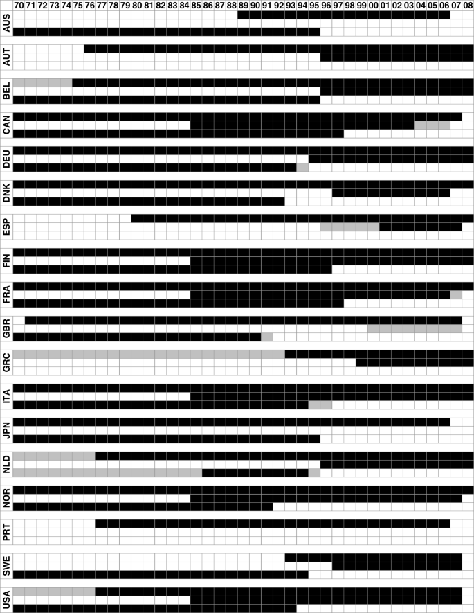
Sectoral productivity data coverage. Notes: For each country, the first row describes the coverage span of the STAN data set; the second, the PDBi; and the third, the ISDB. If all six sectors are available, the line is drawn black, if some sectors are available, it is drawn gray. The STAN data set covers the broadest range of the three data sets
We examine whether there are meaningful differences between the pre-release and the actual release. TFP growth rates of a few countries considered in our baseline estimate slightly differ for some years. Moreover, the coverage also changed to some extent along two dimensions. First, the actual release starts for all countries in 1990, whereas the pre-release contains observations from 1985 onwards for some countries. Second, the public subsector (non-tradable) and the transport, storage, and communications subsector (tradable) are not published, but are available in the pre-release. In order to test whether these differences affect our main findings, we provide a robustness analysis. The results are presented in Table 10 in Appendix 2. We adjust the TFP data set used in our baseline estimation (see column (1) for its result) in three ways. First, we use data of the actual release for all but the two missing subsectors for which we include the pre-release observations (column (2)). Second, we exclude the missing subsectors. Column (3) shows the results with the pre-release data and column (4) shows the results with the actual release. Third, we exclude the missing subsectors but add the business service subsector, which we excluded in our baseline estimate following MacDonald and Ricci (2007) (pre-release: column (5); actual release: column (6)). Most importantly, the differences between the pre-release and actual release do not change the main result of a negative relationship between tradable productivity and the real exchange rate. Not surprisingly, excluding the public subsector (the far largest non-tradable subsector together with the business subsector) leads to insignificant effects of changes in non-tradable productivity on the real exchange rate. However, if we include the business service subsector and exclude the public subsector, the coefficient on productivity in the non-tradable sector becomes significantly negative again.
Therefore, the use of the pre-release in our analysis seems appropriate because of the robustness of the results and two further reasons. First, TFP growth rates in the actual release hardly differ from our pre-release for both the total economy and all published subsectors. This suggests that TFP growth in the two unpublished subsectors are sufficiently close in both releases. Second, the studies using ISDB and/or STAN data from the OECD, and to which we compare our findings, include these subsectors.
-
(v)
OECD, ISDB, Sectoral Productivity Database
The data are from a vintage data set provided by the OECD.
Tradable and non-tradable total factor productivity is calculated for every year t and country i the following way (again, P denotes labor or total factor productivity, and S denotes the share of the subsector):
$$\begin{array}{@{}rcl@{}} P_{i,NT}^{t} & = & \frac{S_{i,{\text{SOC}}}^{t}\cdot P_{i,{\text{SOC}}}^{t} + S_{i,{\text{EGW}}}^{t} \cdot P_{i,{\text{EGW}}}^{t} + P_{i,{\text{CST}}}^{t} \cdot S_{i,{\text{CST}}}^{t} } { S_{i,{\text{SOC}}}^{t} + S_{i,{\text{EGW}}}^{t} + S_{i,{\text{CST}}}^{t} }, \\ P_{i,T}^{t} & = & \frac{S_{i,{\text{AGR}}}^{t} \cdot P_{i,{\text{AGR}}}^{t} + S_{i,{\text{MAN}}}^{t} \cdot P_{i,{\text{MAN}}}^{t} + S_{i,{\text{TRS}}}^{t} \cdot P_{i,{\text{TRS}}}^{t} } { S_{i,{\text{AGR}}}^{t} + S_{i,{\text{MAN}}}^{t} + S_{i,{\text{TRS}}}^{t} }. \end{array} $$Note that SOC: community, social, and personal services; EGW: energy, gas, and water; CST: construction; AGR: agriculture; IND: manufacturing; and TSC: transport, storage, and communications.
-
(vi)
OECD, Unit Labor Costs—Annual Indicators
The data are from the OECD.Stat, available at http://stats.oecd.org/Index.aspx?DataSetCode=ULC_ANN.
-
(vii)
Penn World Tables (PWT)
The data are from the PWT release 7.0. The following variables are used:
-
Real GDP per capita (USD of 2005) (RGDPL)
-
Population (in 1000) (POP)
The population growth rate is calculated as the first difference of the logarithm of POP.
-
-
(viii)
World Bank, World Development Indicators
The following variables are extracted from the WDI CD-ROM:
-
Net foreign assets
Net foreign assets relative to GDP (NFA in the text) is calculated for every year t and country i in the following way:
$$ {\text{NFA}}_{i}^{t} = \frac{{\text{NFA}}_{i,{\text{Level}}}^{t}} {GDP_{i}^{t}\cdot 1000000}$$where NFALevel are the net foreign assets as taken from WDI, and GDP denotes the nominal GDP taken from the OECD Economic Outlook. The missing value of NFALevel for Belgium and France for the year 1998 is replaced by a linearly interpolated value.
-

7 Appendix 2: Additional estimation results
Notes
Rogoff (1996) shows that the speed of adjustment of real exchange rates is too slow to be in line with the PPP theory. Recent studies challenge this finding and stress the importance of non-linear adjustments (Taylor 2003) or dynamic aggregation bias (Imbs et al. 2005). Altogether, the empirical evidence for PPP is mixed (for reviews, see Froot and Rogoff (1996); Taylor (2003) or Gengenbach et al. (2009)
Égert et al. (2006) provide an extensive survey with a focus on transition economies.
However, we also find the results in favor of the BS hypothesis with data from the ISDB.
While Fazio et al. (2007) also use a panel DOLS framework, we also employ a between-dimension group-mean panel FMOLS estimator.
Lee and Tang (2007) and Ricci et al. (2013) also find a negative, though not statistically significant, relationship between productivity of tradables and the real exchange rate. While the result of the former is based on TFP for OECD countries from the ISDB, that of the latter is based on LP calculated using several data sources for a broad range of advanced economies. Focusing on Switzerland, Sax and Weder (2009) and Mancini Griffoli et al. (2015) conclude that changes in sectoral LP do not play a significant role in explaining real exchange rate movements.
For empirical evidence for deviations from the law of one price see, e.g., Engel (1999).
MacDonald and Ricci (2007) and Choudhri and Schembri (2010) provide further results on this mechanism. In contrast, higher productivity in the traded goods sector results in terms of trade improvements and amplifies the Balassa-Samuelson effect in the model developed by Corsetti et al. (2008).
There is no “pricing-to-market” by sellers in their model, and they consider a single currency area.
In the small economy model developed by Devereux (1999), the real exchange rate depreciates because endogenous productivity gains in the service sector lead to a fall in traded goods prices that offsets the BS effect. However, because we exclude the distribution subsector due to classification difficulties (MacDonald and Ricci 2005), this seems not to be the main mechanism that explains the potentially negative relationship between rising productivity in the tradable sector and the real exchange rate in our study. More recently, Bordo et al. (2017) emphasize that the impact of productivity on the real exchange rate varies over time due to changes in trade costs that affect the terms of trade.
All country samples featured in our estimations are presented in Appendix 1.1
In order to verify this claim, we estimate our baseline model with a reference country for each variable. We then re-estimate the same model without using a reference country and obtain identical coefficients and standard errors for all but time fixed effects.
Nonetheless, our main results are robust against the inclusion of the effective real exchange rate (source: OECD Economic Outlook, competitiveness indicator) instead of the unweighted real exchange rate, RER (results not shown).
Note that there are methodological differences compared to the calculated sectoral TFP data in the EU-KLEMS database. For example, whereas in the EU-KLEMS database sectoral TFP is affected by changes in the composition of labor and capital over time, this is not the case for the sectoral TFP data from PDBi used in this paper (Arnaud et al. 2011). However, Arnaud et al. (2011) compare the average TFP change from 1990 to 2007 in manufacturing and services of 13 countries. While average TFP growth is substantially higher in PDBi/STAN compared to EU-KLEMS, the relative TFP growth rates in manufacturing between countries are very similar (except for Ireland, which is excluded in our study), which mainly determines our main finding.
In a robustness analysis, we remove the agriculture subsector from the data set because agriculture is highly protected in some countries (e.g., in Japan).
Adjustments of the threshold value to 5% and 20% leave the division virtually unchanged (De Gregorio and Wolf 1994).
In a robustness analysis, we add the business service subsector to the non-tradable sector at the expense of fewer observations because of its importance for most countries.
In a robustness analysis, we add the distribution subsector to the non-tradable sector.
The advantages are summarized by Canzoneri et al. 1999: first, the labor productivity data are available for more countries and over a longer time period than the TFP numbers. Second, the calculation of LP figures does not require an estimation of the capital stock and the income share of labor, with both estimations likely to be imprecise. Third, the BS hypothesis holds for more technologies than the Cobb-Douglas production function, which is generally employed to determine TFP.
This reflects the use of time-specific dummy variables in all panel estimations. For a brief discussion on the effects of the use of time-specific dummy variables for the choice of the reference country see Section 2.1.
Table 3 IPS and LLC panel unit root test results Non-stationarity of productivity is also consistent with theoretical macroeconomic models (see, e.g., King et al. (1991); Galí (1999) or Lindé (2009)).
The leads and lags remove the correlation between the error term and the stationary component of the non-stationary variables.
As a robustness check, we employ the HC3 estimator proposed by Long and Ervin (2000). The conclusions do not change.
For the theoretical foundation of this methodology, see Pedroni (2004). The conclusions do not change if the residuals are corrected by the estimated leads and lags.
Because of the limited number of observations for every country, we prefer the FMOLS estimator to the DOLS estimator for the group-mean estimations.
To capture the short-run dynamic adjustment of the real exchange rate to temporary disequilibria, an error correction specification is applied to the data. The estimated half-life of deviations of the real exchange rate from its estimated long-run relationship of approximately one to three and a half years, depending on the model specification, is in line with the existing literature.
Notice that due to the lack of data for some years, the coverage is not exactly the same. For the period from 1970 to 2008, Sweden is not covered by the STAN data set. See Figure 2 in Appendix 1 for more details.
We exclude Canada from the sample since there are missing data for Canada from 2004 onwards, which does not affect the conclusions.
Notice that due to the lack of data for some years, the coverage is not exactly the same. See Figure 2 in Appendix 1 for more details.
We also repeatedly re-estimate this specification and each time omit one of the countries. This exclusion exercise reveals that the negative sign is persistent against the omission of any country. In rare cases, the coefficient becomes statistically insignificant.
Table 5 The Balassa-Samuelson effect in recent times For the remaining three countries, TFP.TPDBi is twice insignificantly negative (Austria and Germany) and only once insignificantly positive (Finland).
We repeat this exercise using LP instead of TFP and find a negative coefficient of similar magnitude (− 0.129) on relative sectoral productivity. In this specification, the coefficient is statistically significant at the 10% level.
This is comparable to the countries and years considered by Berka et al. (2018) (see Table 4 of their study). Our sample period ends in 2008 instead of 2009. Moreover, we do not have data on Ireland; for Spain, we only have a small sample size.
One exception is the study by Lee and Tang (2007). The authors use sectoral TFP data from ISDB and find a negative, though not statistically significant, relationship between productivity of tradables and the real exchange rate in their baseline estimation.
As described in Section 2.2, agriculture, manufacturing, and transport, storage, and communications are classified as tradables. If we assume that only manufacturing constitutes the tradable sector, neglecting the other two subsectors, the negative effect is still statistically significant but remains economically small. Focusing on manufacturing might be appropriate since its classification as tradable is the least controversial.
Varying the start point of the estimation sample gradually from 1984 to 1995 does not change the finding of a statistically significant negative coefficient. This result is independent of whether TFP or LP is chosen as a measure of productivity (results not shown)
This finding is also robust to a re-estimation of the model with TFP using only countries in the euro area for the sample period 1995–2008. While the positive coefficient on ULC increases to 0.38 and becomes highly statistically significant, more in line with Berka et al. (2018), the coefficient on TFP.TPDBi declines to − 0.09 but remains statistically significant.
MacDonald and Ricci (2007) and Lee and Tang (2007) include relative wages to control for the indirect effect of a productivity change on the real exchange rate via the wage channel. As a consequence, the direct effect (coefficient on tradable productivity) turns significantly negative.
Notice that Japan is not covered by the PDBi data set.
Note that the absolute price level cannot be identified since the real exchange rate is, by definition, an index due to its computation using the consumer price index (or any other price index).
Fig. 1 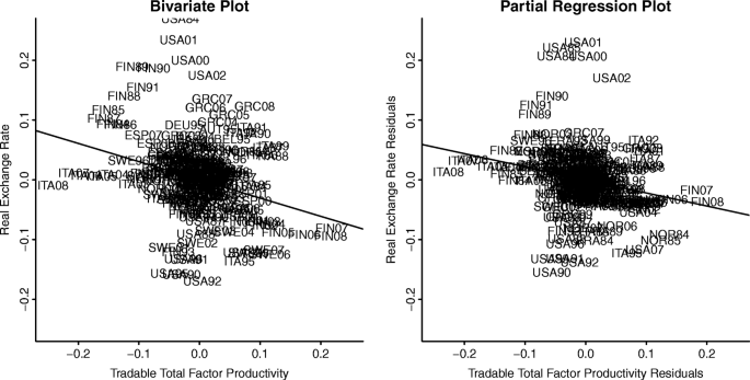
Tradable productivity and the real exchange rate: using data from 1984 to 2008, the plots show the relationship between the real exchange rate and total factor productivity from the OECD productivity database (PDBi). The plots on the left side show the bivariate relationship of the two variables (both the productivity measure and the real exchange rate have been adjusted by country and time fixed effects). The plots on the right side show the results of partial regressions (Velleman and Welsch 1981). On the vertical axis, they show the residuals of a regression of the real exchange rate on the following control variables: non-tradable productivity, terms of trade, country, and time fixed effects. On the horizontal axis, they show the residuals of a regression of productivity in the tradable sector based on the same control variables
For the remaining three countries, TFP.NTPDBi is twice insignificantly negative and once insignificantly positive.

Abbreviations
- AGR:
-
Agriculture
- BS:
-
Balassa-Samuelson
- CA:
-
Current account
- CST:
-
Construction
- DOLS:
-
Dynamic ordinary least squares
- EGW:
-
Energy, gas, and water
- FMOLS:
-
Fully modified ordinary least squares
- DPOP:
-
Population growth
- GDP:
-
Real GDP per capita
- GOV:
-
Government spending
- IND:
-
Manufacturing
- ISDB:
-
International Sectoral Database
- LP:
-
Labor productivity
- LP.T:
-
Labor productivity of tradables
- LP.NT:
-
Labor productivity of non-tradables
- NFA:
-
Net foreign assets
- OECD:
-
Organization for Economic Co-operation and Development
- PDBi:
-
Productivity database by industry
- RER:
-
Real exchange rate
- RI:
-
Long-term real int. rate
- SOC:
-
Community, social, personal services
- STAN:
-
Structural Analysis Database
- TFP:
-
Total factor productivity
- TFP.T:
-
Total factor productivity of tradables
- TFP.NT:
-
Total factor productivity of non-tradables
- TOT:
-
Terms of trade
- TSC:
-
Transport, storage, and communications
- ULC:
-
Unit labor costs
References
Arnaud, B., Dupont, J., Koh, S.-H., Schreyer, P. (2011). Measuring multifactor productivity by industry: Methodology and first results from the OECD productivity database, Technical Report, Organisation for Economic Co-operation and Development.
Balassa, B. (1964). The purchasing-power parity doctrine: a reappraisal. Journal of Political Economy, 72(6), 584–596.
Benigno, G., & Thoenissen, C. (2003). Equilibrium exchange rates and supply-side performance. The Economic Journal, 113(486), 103–124.
Bergin, P.R., Glick, R., Taylor, A.M. (2006). Productivity, tradability, and the long-run price puzzle. Journal of Monetary Economics, 53(8), 2041–2066.
Berka, M., Devereux, M.B., Engel, C. (2018). Real exchange rates and sectoral productivity in the Eurozone. American Economic Review, 108(6), 1543–81.
Bordo, M.D., Choudhri, E.U., Fazio, G., MacDonald, R. (2017). The real exchange rate in the long run: Balassa-Samuelson effects reconsidered. Journal of International Money and Finance, 75, 69–92.
Calderón, C.A. (2004). Real exchange rates in the long and short run: a panel cointegration approach. Revista de Análisis Económico, 19, 41–83.
Canzoneri, M.B., Cumby, R.E., Diba, B. (1999). Relative labor productivity and the real exchange rate in the long run: evidence for a panel of OECD countries. Journal of International Economics, 47(2), 245–266.
Chinn, M.D., & Johnston, L. (1996). Real Exchange Rate Levels, Productivity and Demand Shocks: Evidence from a Panel of 14 Countries, NBER Working Paper 5709. Cambridge: National Bureau of Economic Research.
Choi, I. (2001). Unit root tests for panel data. Journal of International Money and Finance, 20(2), 249–272.
Choudhri, E.U., & Schembri, L.L. (2010). Productivity, the terms of trade, and the real exchange rate: Balassa–Samuelson hypothesis revisited. Review of International Economics, 18(5), 924–936.
Choudhri, E.U., & Khan, M.S. (2005). Real exchange rates in developing countries: are Balassa-Samuelson effects present?IMF Staff Papers, 52(3), 387–409.
Corsetti, G., Dedola, L., Leduc, S. (2008). International risk sharing and the transmission of productivity shocks. The Review of Economic Studies, 75(2), 443–473.
Cribari-Neto, F. (2004). Asymptotic inference under heteroskedasticity of unknown form. Computational Statistics & Data Analysis, 45(2), 215–233.
De Gregorio, J., Giovannini, A., Wolf, H.C. (1994). International evidence on tradables and nontradables inflation. European Economic Review, 38(6), 1225–1244.
De Gregorio, J., & Wolf, H.C. (1994). Terms of Trade, Productivity, and the Real Exchange Rate, NBER Working Paper 4807. Cambridge: National Bureau of Economic Research.
Devereux, M.B. (1999). Real exchange rate trends and growth: a model of East Asia. Review of International Economics, 7(3), 509–521.
Driscoll, J.C., & Kraay, A.C. (1998). Consistent covariance matrix estimation with spatially dependent panel data. Review of Economics and Statistics, 80(4), 549–560.
Égert, B., Lommatzsch, K., Lahrèche-Révil, A. (2006). Real exchange rates in small open OECD and transition economies: Comparing apples with oranges?Journal of Banking & Finance, 30(12), 3393–3406.
Égert, B., Halpern, L., MacDonald, R. (2006). Equilibrium exchange rates in transition economies: taking stock of the issues. Journal of Economic Surveys, 20(2), 257–324.
Engel, C. (1999). Accounting for US real exchange rate changes. Journal of Political Economy, 107(3), 507–538.
Fazio, G., McAdam, P., MacDonald, R. (2007). Disaggregate real exchange rate behaviour. Open Economies Review, 18(4), 389–404.
Froot, K.A., & Rogoff, K. (1996). Perspectives on PPP and Long-Run Real Exchange Rates, NBER Working Paper 4952. Cambridge: National Bureau of Economic Research.
Galí, J. (1999). Technology, employment, and the business cycle: do technology shocks explain aggregate fluctuations?American Economic Review, 89(1), 249–271.
Gengenbach, C., Palm, F.C., Urbain, J.-P. (2009). Panel unit root tests in the presence of cross-sectional dependencies: Comparison and implications for modelling. Econometric Reviews, 29(2), 111–145.
Gubler, M., & Sax, C. (2014). Skill-biased technological change and the real exchange rate, SNB Working Paper 2014-09.
Harris, D., Leybourne, S., McCabe, B. (2005). Panel stationarity tests for purchasing power parity with cross-sectional dependence. Journal of Business & Economic Statistics, 23(4), 395–409.
Harrod, R.F. (1933). International Economics. Cambridge Economic Handbooks. London: Nisbet & Cambridge University Press.
Im, K.S., Pesaran, M.H., Shin, Y. (2003). Testing for unit roots in heterogeneous panels. Journal of Econometrics, 115(1), 53–74.
Imbs, J., Mumtaz, H., Ravn, M.O., Rey, H. (2005). PPP strikes back: aggregation and the real exchange rate. The Quarterly Journal of Economics, 120(1), 1–43.
Kao, C. (1999). Spurious regression and residual-based tests for cointegration in panel data. Journal of Econometrics, 90(1), 1–44.
Kao, C., & Chiang, M.-H. (2001). On the estimation and inference of a cointegrated regression in panel data. In: Carter Hill, R., Baltagi, B.H., Fomby, T.B. (Eds.) In Nonstationary Panels, Panel Cointegration, and Dynamic Panels, Vol. 15 of Advances in Econometrics. chapter 7. Emerald Group Publishing Limited, (pp. 179–222).
King, R.G., Plosser, C.I., Stock, J.H., Watson, M.W. (1991). Stochastic trends and economic fluctuations. American Economic Review, 81(4), 819–840.
Krugman, P. (1990). Equilibrium exchange rates. In: Branson, W.H., Frenkel, J.A., Goldstein, M. (Eds.) In International Policy Coordination and Exchange Rate Fluctuations. The University of Chicago Press.
Lane, P.R., & Milesi-Ferretti, G.M. (2004). The transfer problem revisited: Net foreign assets and real exchange rates. Review of Economics and Statistics, 86(4), 841–857.
Lee, J., & Tang, M.-K. (2007). Does productivity growth appreciate the real exchange rate?Review of International Economics, 15(1), 164–187.
Levin, A., Lin, C.-F., Chu, C.-S.J. (2002). Unit root tests in panel data: asymptotic and finite-sample properties. Journal of Econometrics, 108(1), 1–24.
Lindé, J. (2009). The effects of permanent technology shocks on hours: can the RBC-model fit the VAR evidence?Journal of Economic Dynamics and Control, 33(3), 597–613.
Long, J.S., & Ervin, L.H. (2000). Using heteroscedasticity consistent standard errors in the linear regression model. The American Statistician, 54(3), 217–224.
MacDonald, R., & Ricci, L.A. (2005). The real exchange rate and the Balassa–Samuelson effect: the role of the distribution sector. Pacific Economic Review, 10(1), 29–48.
MacDonald, R., & Ricci, L.A. (2007). Real exchange rates, imperfect substitutability, and imperfect competition. Journal of Macroeconomics, 29(4), 639–664.
Maddala, G.S., & Wu, S. (1999). A comparative study of unit root tests with panel data and a new simple test. Oxford Bulletin of Economics and Statistics, 61(S1), 631–652.
Mancini Griffoli, T., Meyer, C., Natal, J.-M., Zanetti, A. (2015). Determinants of the Swiss franc real exchange rate. Swiss Journal of Economics and Statistics, 151(4), 299–331.
Ng, S., & Perron, P. (2001). Lag length selection and the construction of unit root tests with good size and power. Econometrica, 69(6), 1519–1554.
Pedroni, P. (2001). Purchasing power parity tests in cointegrated panels. Review of Economics and Statistics, 83(4), 727–731.
Pedroni, P. (2004). Panel cointegration: asymptotic and finite sample properties of pooled time series tests with an application to the PPP hypothesis. Econometric Theory, 20(03), 597–625.
Pesaran, M.H. (2007). A simple panel unit root test in the presence of cross-section dependence. Journal of Applied Econometrics, 22(2), 265–312.
Ricci, L.A., Milesi-Ferretti, G.M., Lee, J. (2013). Real exchange rates and fundamentals: A Cross-Country Perspective. Journal of Money, Credit and Banking, 45(5), 845–865.
Rogoff, K. (1996). The purchasing power parity puzzle. Journal of Economic Literature, 19, 647–668.
Rose, A.K., Supaat, S., Braude, J. (2009). Fertility and the real exchange rate. Canadian Journal of Economics/Revue canadienne d’économique, 42(2), 496–518.
Samuelson, P. (1964). Theoretical notes on trade problems. Review of Economics and Statistics, 46(2), 145–154.
Sax, C., & Weder, R. (2009). How to explain the high prices in Switzerland?Swiss Journal of Economics and Statistics, 145(4), 463–483.
Stein, J.L., & Allen, P.R. (1997). Fundamental determinants of exchange rates. USA: Oxford University Press.
Stock, J.H., & Watson, M.W. (1993). A simple estimator of cointegrating vectors in higher order integrated systems. Econometrica, 61(4), 783–820.
Taylor, M.P. (2003). Purchasing power parity. Review of International Economics, 11(3), 436–452.
Tica, J., & Družić, I. (2006). The Harrod-Balassa-Samuelson effect: a survey of empirical evidence. University of Zagreb, Faculty of Economics and Business, FEB–Working Paper Series (No. 06-7/686).
Tintin, C. (2014). Does the Balassa-Samuelson hypothesis still work? Evidence from OECD countries. International Journal of Sustainable Economy, 6(1), 1–18.
Velleman, P.F., & Welsch, R.E. (1981). Efficient computing of regression diagnostics. The American Statistician, 35(4), 234–242.
Acknowledgements
Without reservation, we would like to thank Sylvia Kaufmann, Markus Ludwig, Christian Rutzer, Linda Walter, Rolf Weder, two anonymous reviewers and the seminar participants at the University of Basel for their helpful comments and suggestions, as well as the OECD for kindly sharing two essential data sets on sectoral productivity. Hermione Miller-Moser provided excellent editorial assistance. Matthias Gubler is indebted to Peter Kugler for his help and supervision. Christoph Sax acknowledges support from the WWZ Forum Foundation. The views expressed in this paper are those of the authors and do not necessarily reflect those of the SNB.
Funding
Christoph Sax acknowledges support from the WWZ Forum Foundation. The funding source (WWZ Forum Foundation) had no involvement in study design; in the collection, analysis and interpretation of data; in the writing of the report; and in the decision to submit the paper for publication.
Availability of data and materials
All but two data sets used and/or analysed during the current study are available from the corresponding author on reasonable request. The pre-release of the OECD productivity database with sectoral productivity data (PDBi, ISIC Rev. 3 version) and International Sectoral Database (ISDB) are available from the authors upon reasonable request and with permission of the OECD.
Author information
Authors and Affiliations
Contributions
All authors were equally involved in the design and empirical analysis of this project. All authors read and approved the final manuscript.
Corresponding author
Ethics declarations
Competing interests
The authors declare that they have no competing interests.
Publisher’s Note
Springer Nature remains neutral with regard to jurisdictional claims in published maps and institutional affiliations.
Rights and permissions
Open Access This article is distributed under the terms of the Creative Commons Attribution 4.0 International License (http://creativecommons.org/licenses/by/4.0/), which permits unrestricted use, distribution, and reproduction in any medium, provided you give appropriate credit to the original author(s) and the source, provide a link to the Creative Commons license, and indicate if changes were made.
About this article

Cite this article
Gubler, M., Sax, C. The Balassa-Samuelson effect reversed: new evidence from OECD countries. Swiss J Economics Statistics 155, 3 (2019). https://doi.org/10.1186/s41937-019-0029-3
Received:
Accepted:
Published:
DOI: https://doi.org/10.1186/s41937-019-0029-3